
A chi square test in research checks whether two categorical variables are associated, such as level of study and whether students use a service. It compares the counts you observed in each cell of a table with the counts you would expect if the variables were unrelated. A large gap gives a small p-value.
Once your numbers are checked, the write-up still has to be clear and consistent. UniDraft organises your confirmed results, checked sources and supervisor instructions into an editable Word document. Start your project document when your analysis is ready, and keep your software output beside the draft. UniDraft does not run the test for you. If you are still deciding which test suits your objective, read which statistical test fits your final year project first, then come back here for the chi square detail.
What does the chi square test of independence actually do?
Imagine a table with levels of study down the side and "uses the e-resource portal: yes or no" across the top. Each cell holds a count of students. If level of study made no difference to portal use, the proportion of "yes" would be about the same in every row. The test works out how many students you would expect in every cell under that "no difference" idea, then measures how far your real counts are from those expectations.
The distance is summarised in one number, the chi square statistic, written χ². Each cell contributes (observed − expected)² ÷ expected, and you add the contributions. A bigger χ² means a bigger overall gap. Software turns it into a p-value using the degrees of freedom of your table.
This is the chi square test of independence (some books call it the test of association). It is not the only chi square test. The goodness-of-fit version compares one variable's counts with a claimed pattern, for example whether responses are spread equally across four options. Most Chapter 4 questions about "is A related to B" need the independence version, so that is what this guide covers.
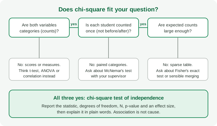
When does a chi square test fit your project?
Check three things before you reach for it.
- Both variables are categories. Faculty, gender, level, yes/no, state of origin, type of placement. If one variable is a measurement such as a score or time in minutes, you probably need a different tool; the correlation table guide covers relationships between two measurements.
- Each respondent appears once. Kent State University's SPSS guide lists independent observations as an assumption: each subject appears once and the variables are not paired, as in a before-and-after design. For paired categories it points to McNemar's test instead.
- The sample is large enough for the expected counts. More on this below, because students often misread the rule.
A good chi square question reads like this: "Is use of the library portal associated with level of study?" or "Is choice of placement type associated with gender?" A poor fit: "Did the training improve scores?" (a measurement, measured twice) or "How many students use the portal?" (a count and percentage is the whole answer).
Notice that the test needs your variables to be categories by design. If you planned to collect ages as numbers and later group them into bands, that is allowed, but decide the bands from your objectives and a sensible literature or supervisor convention before you look at the results. Choosing bands to manufacture significance is a common and avoidable mistake. The way your questionnaire records each variable decides what you can do later, so check this before data collection, not after.
How do you write the hypotheses?
For a test of independence the hypotheses follow a fixed pattern. Kent State's guide words them as: the null hypothesis says the two variables are independent (not associated), and the alternative says they are not independent (associated).
In a project you attach the actual variables:
- H0: There is no association between level of study and use of the e-resource portal.
- H1: There is an association between level of study and use of the e-resource portal.
Two notes. First, the chi square test of independence is not directional by itself. It can say "these are associated", but it does not say which row has a higher rate until you look at the table of percentages. If your department insists on directional hypotheses, discuss the right test with your supervisor. Second, hypotheses should be written before analysis and should match your objectives. Our guide to writing hypotheses for a final year project shows the wording, and the research questions and objectives guide shows how each hypothesis traces back to an objective.
Also fix your significance level in Chapter 3 (many projects use 0.05, but follow your department). The decision rule is then simple: if p is below your chosen level, reject H0 and conclude there is evidence of an association; otherwise you do not have enough evidence of one. "Not enough evidence" is different from "proved there is no relationship".
What is the expected count assumption?
This is the part most often misunderstood.
An expected count is the number of respondents a cell would hold if the variables were independent. You calculate it as:
expected = (row total × column total) ÷ grand total
The rule of thumb is about these expected counts. Kent State's guide says expected frequencies should be at least 5 for the majority (80%) of the cells, and at least 1 for every cell. SPSS prints a footnote under the output table telling you how many cells fall below 5 and the smallest expected count, so look at it every time. The Analysis Factor makes the same point strongly: the rule is not about how many students are in each observed cell. You can have an observed cell of 2 and still be fine if its expected count is above the limit.
Textbooks and websites do not all use the same cut-off. Some are stricter and some looser, which is why you should treat "5" as a common guide and confirm what your supervisor or department expects. This guide gives no universal number beyond what those sources state.
If expected counts are too small, your options, according to the sources opened for this guide, include:
- Fisher's exact test, which does not rely on the chi square approximation and is the usual alternative for small tables (Navarro and Foxcroft's textbook chapter, and The Analysis Factor).
- Combining categories when it makes substantive sense, for example merging two sparse levels that your literature already treats together. Decide this on meaning, not on which merge gives the lowest p-value.
- A continuity correction for some 2×2 tables, which The Analysis Factor attributes to Cochran for expected counts from 5 to under 10. Whether your software applies it by default varies, so state which one you used.
The other assumption is independence: no student counted twice, no copied or group-filled forms, no paired design. Violating it cannot be fixed by a bigger sample. This is also why your sampling approach matters. A chi square p-value does not make a convenience sample random.
A worked example you can check by hand
Everything below is fictional and invented to show the arithmetic. It is not a real survey and not a real result.
Objective (illustrative): examine whether use of a library e-resource portal is associated with level of study.
Data (illustrative): 240 students, 80 each from 200, 300 and 400 level, asked whether they used the portal this semester.
| Level | Used the portal | Did not use | Row total | % who used |
|---|---|---|---|---|
| 200 level | 30 | 50 | 80 | 37.5% |
| 300 level | 45 | 35 | 80 | 56.3% |
| 400 level | 55 | 25 | 80 | 68.8% |
| Column total | 130 | 110 | 240 |
Step 1: hypotheses. H0: level of study and portal use are independent. H1: they are associated. Significance level 0.05.
Step 2: expected counts. For the "used" column, each row gives 80 × 130 ÷ 240 = 43.33. For the "did not use" column, 80 × 110 ÷ 240 = 36.67. Because every row has 80 students, the expected counts are the same in each row. All six expected counts are well above 5, so the assumption is comfortably met.
Step 3: contributions to χ². Each cell gives (O − E)² ÷ E:
| Cell | Observed | Expected | (O − E)² ÷ E |
|---|---|---|---|
| 200, used | 30 | 43.33 | 4.10 |
| 200, not used | 50 | 36.67 | 4.85 |
| 300, used | 45 | 43.33 | 0.06 |
| 300, not used | 35 | 36.67 | 0.08 |
| 400, used | 55 | 43.33 | 3.14 |
| 400, not used | 25 | 36.67 | 3.71 |
Adding them gives χ² ≈ 15.94. The arithmetic was checked by computing it with a short script, and the figures above agree with it.
Step 4: degrees of freedom. df = (rows − 1) × (columns − 1) = (3 − 1) × (2 − 1) = 2. This matches the formula Kent State's guide uses.
Step 5: p-value. With 2 degrees of freedom the upper-tail probability is e^(−χ²/2), which gives about 0.0003 here, so p < .001. Software will print the same thing. Since p is below 0.05, reject H0.
Step 6: effect size. Significance does not say how strong the association is. One common measure is Cramér's V, which is √(χ² ÷ (N × (k − 1))) where k is the smaller of the number of rows and columns. Here k = 2, so V = √(15.94 ÷ 240) ≈ 0.26. Sources give different verbal labels for small, medium and large values, so report the number and use the label your department prefers rather than copying one from a website.
Step 7: look at the pattern. The test says the variables are associated, but the table of row percentages tells the story: the share of students using the portal rises from 37.5% at 200 level to 68.8% at 400 level, and the largest contributions to χ² come from the 200-level and 400-level rows. That is the sentence your discussion needs.
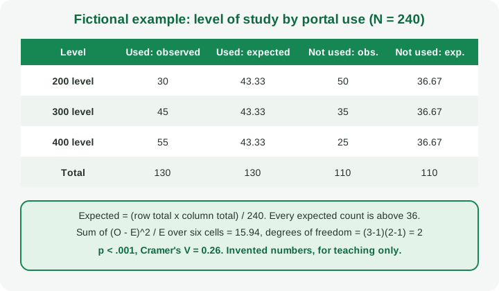
You do not need to do this by hand in your real project; software does it. But once you have done it by hand with a small table, the SPSS or Excel output stops being a mystery and you can answer a panel member who asks where the number came from.
How do you read and report the result in Chapter 4?
Present three things in order: the table, the test, and the meaning.
1. The table. Show observed counts with row percentages, so the reader can see the pattern. Give it a numbered caption and a source line saying it comes from your field survey. The format figures, tables and captions guide covers captions and placement.
2. The test. A common reporting pattern gives the statistic, degrees of freedom, sample size, p-value and effect size. For the fictional example:
A chi-square test of independence indicated an association between level of study and use of the e-resource portal, χ²(2, N = 240) = 15.94, p < .001, Cramér's V = 0.26. All expected counts exceeded 5.
State that you checked the expected counts, and say which correction or alternative test you used if the table needed it. Your department may want a different style or a table of test results instead of a sentence, so follow its guidance.
3. The meaning. Tie the result back to the hypothesis and the objective in plain language: "The null hypothesis of no association is rejected. The proportion using the portal was higher among students in higher levels." Stop there in Chapter 4. Explaining why belongs in the discussion, where you compare with your literature and admit limits; see the Chapter 5 guide. For the overall layout of results, the Chapter 4 guide shows how to organise tables, test results and commentary without pasting raw software output.
If the result is not significant, report it with the same care. "No evidence of an association was found at the 0.05 level" is a legitimate finding, and you should not keep re-cutting the categories until something crosses the line.
Common chi square mistakes supervisors flag
- Using percentages instead of counts in the calculation. The test needs raw counts of respondents.
- Applying the "5" rule to observed cells. The rule is about expected counts.
- Ignoring a warning footnote in the software output about cells with small expected counts, and reporting the p-value anyway.
- Merging categories after seeing the result so that the p-value drops.
- Using the test on paired or repeated data, such as the same students before and after, or the same person counted in two rows.
- Treating significance as strength. A small p-value with a very large sample can sit beside a weak association; that is why an effect size helps.
- Claiming causation. Kent State's guide is explicit that the test shows association, not causation.
- Running chi square on a Likert-scale average or any measured score. A single Likert item can be tabulated as categories, but check with your supervisor whether another approach suits ordered responses; see Likert scale analysis.
- Testing every pair of variables and reporting only the significant ones. Decide the tests from your objectives first.
- Too many empty categories. A 6 × 5 table from a sample of 80 will almost certainly have sparse cells. Plan the number of categories before you collect data.
Questions a panel might ask
- Why did you choose a chi square test and not a t-test?
- Are your variables categorical, and how were they coded?
- What are your hypotheses, and what was your significance level?
- How did you check the expected counts?
- What does the p-value mean, and does it tell us the strength of the association?
- Can you say that level of study causes portal use?
- What would you do if some cells were too small?
If you can answer these from your own table, you understand your analysis. Practise with the defence questions guide alongside it.
Checklist before Chapter 4
- The objective and both hypotheses are written, and the test is named in Chapter 3.
- Both variables are categories, with coding recorded in your codebook (see coding and cleaning questionnaire data).
- Each respondent is counted once.
- You looked at the expected counts, not only the observed counts.
- The table shows counts and row percentages.
- You report χ², degrees of freedom, N, p and an effect size if required.
- Your interpretation says "associated", not "caused".
- Your supervisor or departmental statistician has seen the output.
When your analysis is confirmed, UniDraft can help you organise the verified results, your checked sources and your supervisor's instructions into an editable Word document. Start your project document. You can also use the free citations tool for your sources and the formatter to check layout.
Sources
- Kent State University Libraries: Chi-square test of independence: assumptions, hypotheses, expected-frequency rule, degrees of freedom, association not causation.
- Navarro and Foxcroft, Learning Statistics with jamovi: assumptions of the chi-square tests: expected frequencies, independence, Fisher exact test.
- The Analysis Factor: Chi-square test of independence rule of thumb: the rule applies to expected counts; alternatives for small counts.